Understanding the math behind HRM

One of my favorite papers is HRM by Sapient Intelligence, and I dug deep into its math a while back. I found two things interesting, first: a lot of my early NLP days was figuring out recursive modules like lstms, which dont find much use nowadays; second: they claimed bio inspiration which I am fond of.

About half a year back, I presented this to my cofounders. I thought it would be nice to revise, and have an online record of it. I plan to focus on the motivation for it, and the core math as inferred from the contents of the paper.

If I have gotten something wrong, please email me so I can correct it.

Why Transformers are not enough.

Transformers, and the LLMs built on them, are inherently shallow. Computation happens in a single forward pass of fixed depth, so there’s a hard ceiling on how much “thinking” can happen before an answer has to come out. It does not perform well enough for tough reasoning tasks.

A way around this is Chain of Thought (CoT) prompting. In this, reasoning follows the same process as humans, writing down step by step the prioirs, reasons, and then the execution. Ultimately, its just a way around the shortcomings, not the best solution.

There are issues with CoT too, it depends on human defined reasoning steps, and any mistake means that you are stuck with that block for the whole pass. Also, tokens are too ineffecient to think in, to which there was COCONUT (Chain of Continuous Thought) that replaced tokens with thought tokens. This too is not good enough.

Why is Computational Depth important?

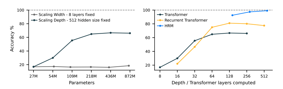
In the left-graph, on Sudoku-Extreme Full, which require extensive tree-search and backtracking, increasing a Transformer’s width yields no performance gain, while increasing depth is critical. The graph on the right shows how HRM is able to achieve better performance even than recursive transformers, highlighting that there is a ceiling on recurrant transformers.

Naively stacking layers is notoriously poor due to vanishing gradients, which cause poor training stability and ineffectiveness (something which RNNs faced). It is also insanely expensive computationally due to lack of parallelisation possible, both in forward pass and in backward. This is due to BPTT (backpropagation through time).

HRM Architecture

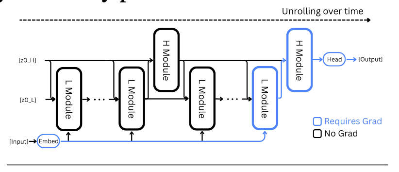
There are multiple parts of HRM architecture which I will go one by one. The main one though is the diagram above. The two-layer hierarchical recursive neural network. Here, each recursive unit is in itself a transformer.

The logic is simple: the low-level RNN unrolls for \(N\) steps, after which the high-level RNN updates. This happens \(T\) times. There is not much to think here wrt architecture, but the math of it is interesting.

There are four neural layers: Input \(I\), Low-Level RNN \(L\), High-Level RNN \(H\), and Output \(O\).

$$ \begin{aligned} \text{I} &= f_I(;\theta_I) \\ \text{L} &= f_L(;\theta_L) \\ \text{H} &= f_H(;\theta_H) \\ \text{O} &= f_O(;\theta_O) \end{aligned} $$

Each of these functions take inputs as the following

$$ \begin{aligned} \widetilde{x} &= f_I(x; \theta_I) \\ z_{L}^{i} &= f_L(z_{L}^{i-1}, z_{H}^{i-1}, \widetilde{x}; \theta_L) \\ z_{H}^{i} &= \begin{cases} f_H(z_{L}^{i}, z_{H}^{i-1}; \theta_H) & i \equiv 0 \pmod{T} \\ z_{H}^{i-1} & \text{otherwise} \end{cases} \\ \widehat{y} &= f_O(z_{H}^{i}; \theta_O) \end{aligned} $$

All of this is fairly simple initialisations in math. The input and output layers are straightforward, while the recursive units are take each other as input params.

Now, for the 1-step BPTT algorithm.

Assumption: Consider an idealised HRM behaviour.

Here, $$ z_{L} \to z_{L}^{*} $$

Essentially, \(z_{L}\) converges over the lower-level RNN iterations at some \(k-1\) th higher-level RNN step.

$$ z_{L}^{*} = f_L(z_{L}^{*}, z_{H}^{k-1}, \widetilde{x}; \theta_L) \tag{1} $$

then,

$$ z_{H}^{k} = f_H(z_{L}^{*}, z_{H}^{k-1}; \theta_H) \tag{2} $$

You can compress this into a single Function

$$ z_{H}^{k} = \mathcal{F}(z_{H}^{k-1}, \widetilde{x}; \theta) \\ \theta = (\theta_I, \theta_L, \theta_H) $$

So, you get

$$ z_{H}^{*} = \mathcal{F}(z_{H}^{*}, \widetilde{x}; \theta) \tag{3} $$

Implicit Function Theorem

The Implicit Function Theorem tells how to represent one variable as a function of others, even if the relationship between them is given implicitly.

Let’s say I have a curve such that \(f(x, y) = 0\) for some \(x_0\) and \(y_0\).

We then find a nearby point on the same curve such that $$ f(x_0, y_0) = 0 \\ f(x_0 + \Delta{x}, y_0 + \Delta{y}) = 0 $$

We then use Taylor Expansion for two variables:

$$ f(x + a, y + b) = f(x, y) + \frac{\partial{f}}{\partial{x}}(a) + \frac{\partial{f}}{\partial{y}}(b) . . . $$

In our case, we get

$$ f(x_0 + \Delta{x}, y_0 + \Delta{y}) = f(x_0, y_0) + \frac{\partial{f}}{\partial{x}}(\Delta{x}) \bracevert_{x_0, y_0} + \frac{\partial{f}}{\partial{y}}(\Delta{y}) \bracevert_{x_0, y_0} . . . $$

Since \(\Delta{x}\) and \(\Delta{y}\) are small, we can approximate using first-order Taylor expansion.

Also, we know that \(f(x_0 + \Delta{x}, y_0 + \Delta{y}) = 0\) and \(f(x_0, y_0) = 0\), so

$$ \frac{\Delta{y}}{\Delta{x}} = \frac{\frac{\partial{f}}{\partial{x}}}{\frac{\partial{f}}{\partial{y}}} \bracevert_{x_0, y_0} = - \frac{f_x}{f_y} $$

Note, \(f_x\) and \(f_y\) are still the same partial derivatives, I am just using different variables to represent it.

As \(\Delta \to 0\), we get

$$ \frac{dy}{dx} = - \frac{f_x}{f_y} \bracevert_{x_0, y_0} \tag{4} $$

Gradient Approximation

We had, from equation (3), that

$$ z_{H}^{*} = \mathcal{F}(z_{H}^{*}, \widetilde{x}, \theta) = \mathcal{F}(z_{H}^{*}, \theta) $$

Let’s say

$$ g(z_{H}^{*}, \theta) = z_{H}^{*} - \mathcal{F}(z_{H}^{*}, \theta) $$

Using Implicit Function Theorem from equation (4), we get

$$ \frac{dz_{H}^{*}}{d\theta} = - \frac{g_{\theta}}{g_{z_{H}^{*}}} \bracevert_{z_{H}^{*}} \tag{5} $$

Where

$$ g_{\theta} = \frac{\partial{g}}{\partial{\theta}} = 0 - \frac{\partial{\mathcal{F}}}{\partial{\theta}} = - \frac{\partial{\mathcal{F}}}{\partial{\theta}} \bracevert_{z_{H}^{*}} \tag{6} $$

and

$$ g_{z_{H}^{*}} = \frac{\partial{g}}{\partial{z_{H}^{*}}} = I - \frac{\partial{\mathcal{F}}}{\partial{z_{H}^{*}}} \bracevert_{z_{H}^{*}} $$

Here, obviously, \(I\) is the identity matrix. We also know that \(\frac{\partial{\mathcal{F}}}{\partial{z_{H}^{*}}}\) is also the Jacobian of \(\mathcal{F}\) with respect to \(z_{H}^{*}\).

So, we get

$$ g_{z_{H}^{*}} = I - J_{\mathcal{F}}\bracevert_{z_{H}^{*}} \tag{7} $$

Replacing equations (6) and (7) in equation (5), we get

$$ \frac{dz_{H}^{*}}{d\theta} = (I - J_{\mathcal{F}})^{-1} \frac{\partial{\mathcal{F}}}{\partial{\theta}} \bracevert_{z_{H}^{*}} \tag{8} $$

To reflect, the term \(\frac{\partial{z_{H}^{*}}}{\partial{\theta}}\) is the BPTT term. Normally, we have to roll it back all the way to \(z_{H}^0\) for BPTT, but here we will do some approximation soon to get it value in single-shot.

Neumann Series Expansion

Neumann Series Expansion of Matrix gives us

$$ (I - A)^{-1} = \sum_0^{\inf} A^k \tag{9} $$

Lets take the function

$$ z_{H}^{k+1} = \mathcal{F}(z_{H}^{k}) \tag{10} $$

If we do Taylor Series Expansion over this function around \(z_{H}^{*}\), we get:

$$ \mathcal{F}(z_{H}^{k}) = \mathcal{F}(z_{H}^{*}) + J_{\mathcal{F}}(z_{H}^{k} - z_{H}^{*}) $$

Using Equation (10) on this, we get

$$ z_{H}^{k+1} = z_{H}^{*} + J_{\mathcal{F}}(z_{H}^{k} - z_{H}^{*}) $$

Which can be written as

$$ \delta{z_{H}^{k+1}} = J_{\mathcal{F}}(\delta{z_{H}^k}) \tag{11} $$

Now, lets write it down for all \(k\) starting from 0:

$$ \delta{z_{H}^1} = J_{\mathcal{F}}\cdot(\delta{z_{H}^0}) \tag{k=0} $$

$$ \delta{z_{H}^2} = J_{\mathcal{F}}\cdot (\delta{z_{H}^1}) \\ \tag{k=1} \delta{z_{H}^2} = J_{\mathcal{F}}^2 \cdot \delta{z_H^0} $$

As we continue unrolling \(k\), we get a general formula

$$ \delta{z_{H}^k} = J_{\mathcal{F}}^k\cdot\delta{z_H^0} \tag{12} $$

When convergence happens, \(\delta{z_H^k} \to 0\). Based on (12), this means that \(J_{\mathcal{F}} \to 0\) as well. This is only possible when \(J_{\mathcal{F}} \lt 1 \).

This is a really important result, since now we can use (9), but this time we ignore all terms except \(k=0\), since anyway \(J_{\mathcal{F}} \lt 1\). This is an approximation, not assumption, but it doesnt change much in terms of complexity. If you want to be pedantic and take k till some arbitrary value (or even to the number of rollouts), you can, but this equation proves that approximating it by not considering them is valid.

HRM Final Equations

Using (9) now, we can re-write equation (8) as:

$$ \frac{dz_{H}^{*}}{d\theta} = I \cdot \frac{\partial{\mathcal{F}}}{\partial{\theta}} \bracevert_{z_{H}^{*}} $$

Removing the compressed functions, we get $$ \frac{dz_{H}^{*}}{d\theta_H} = \frac{df_H}{d\theta_H} \bracevert_{z_{H}^{*}} \tag{13} $$

and $$ \frac{dz_{H}^{*}}{d\theta_L} = \frac{df_H}{d\theta_L} = \frac{df_H}{dz_{L}^{*}} \cdot \frac{dz_{L}^{*}}{d\theta_L} \tag{14} $$

and $$ \frac{dz_{H}^{*}}{d\theta_I} = \frac{df_H}{d\theta_I} = \frac{df_H}{dz_{L}^{*}} \cdot \frac{dz_{L}^{*}}{d\theta_I} \tag{15} $$

It is very easy to resolve the \(\frac{dz_{L}^{*}}{d\theta}\) term in both (14) and (15), since we just use the same approximations again to get: $$ \frac{dz_{H}^{*}}{d\theta_L} = \frac{df_H}{d\theta_L} = \frac{df_H}{dz_{L}^{*}} \cdot \frac{df_{L}}{d\theta_L} \bracevert_{z_{L}^{*}, z_{H}^{*}} \tag{14} $$

So boom, we are done with the approximation of BPTT. Now we have a one-shot way to calculate the gradients.

Deep Supervision

HRM is completely built on this iteration. Since they have avoidede the computational cost of BPTT, they try to maximise the number of iterations they can. From this is born the idea of Deep Supervision.

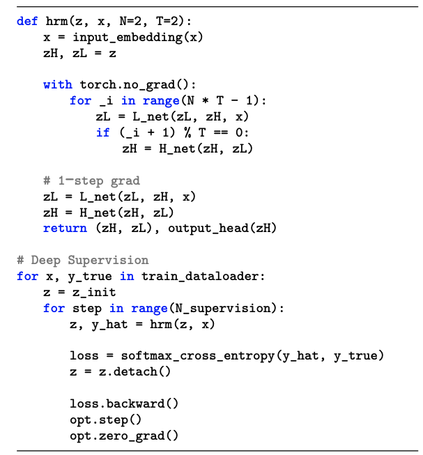
The code is more or less self-explanatory. For each data sample \((x, y)\), we iter over the hrm-network \(N_{\text{supervision}}\) times (or, to say it easier, \(M\) times). Crucially, the hidden state \(z^m\) is detached from the computation graph before being used as the input for next segment. Hence, the gradients do not propagate back through segment \(m\), effectively creating a 1-step approximation here as well.

Adaptive Computational Time (ACT)

Having so much iterations, even with 1-step approximations, adds up in cost. Especially in training when there are certain modules which have been answered earlier, and now you are stuck repeating 5-6 more deep supervision iteration. For this, HRM introduces ACT to adaptively determine the number of segments.

The do this by using a DQN (Deep Q Network), which uses the Q head on the final state of the H-module to determine Q-Values.

$$ \widehat{Q}^m = (\widehat{Q}^m_{\text{halt}}, \widehat{Q}^m_{\text{continue}}) $$

To draw simple parallel to traditional Q learning, the state is \(z^{mNT}_H\), and we must find the best possible action between halt and continue. To do so, in traditional model-free method, we determine Q values of the two action given the state.

$$ \widehat{Q}^m = \sigma(\theta_Q \cdot z_{H}^{mNT}) $$

They dont let Q learning take all the decisions though, there are some safe checks in place. The halt or continue action is chosen using random strategy. Let \(M_{\text{max}}\) is max num of segments, and \(M_{\text{min}}\) num of segments before it can halt. \(M_{\text{min}}\) is chosen stochastically as follows: $$ M_{\text{min}} = \begin{cases} \text{uniform from} \{2, . . , M_{\text{max}}\} & \epsilon \\ 1 & 1 - \epsilon \end{cases} $$

Halt happens either when segment count surpasses \(M_{\text{max}}\) or if \(\widehat{Q}^m_{\text{halt}} \gt \widehat{Q}^m_{\text{continue}}\).

The Q network is a NN too, and it must be trained to produce good quality answers. We do this in a simple 1-step future look-ahead manner. We get the targets \(\widehat{G}^m\) as:

$$ \widehat{G}^m_{\text{halt}} = 1\{\widehat{y}^m = y\} $$

$$ \widehat{G}^m_{\text{continue}} = \begin{cases} \widehat{Q}^{m+1}_{\text{halt}} & \text{if } m \geq M_{\text{max}}\\ max(\widehat{Q}^{m+1}_{\text{halt}}, \widehat{Q}^{m+1}_{\text{continue}}) & \text{otherwise} \\ \end{cases} $$

Loss for this is simply calculated as $$ L^m_{\text{ACT}} = \text{LOSS}(\widehat{y}^m, y) + \text{BinaryCrossEntropy}(\widehat{Q}^m, \widehat{G}^m) $$

To get the Q values at m+1 time, we do another forward pass, use those values, then do the loss calculation against it.

References

Hierarchical Reasoning Model: All of the diagrams and understanding is via this. They have done a pretty good job explaining what is happening (also made code public!)

I also used claude and Wiki a bit to understand a few steps here and there.